Single Shot MultiBox Detector(SSD)

2022 Open Source Contribution Academy 의 Pytorch Hub 번역 팀의 일원으로 Single Shot MultiBox Detector(SSD) 논문에 대한 정리 및 예제 모델 학습을 해보았습니다.

논문 배경 상황 설명

SSD는 Object Detection을 목표로 ECCV’ 16에 게제된 Paper 입니다.

arxiv에는 2015/12월에 게제 되었으며, 근처에 나온 관련 논문으로는 Fast R-CNN (ICCV' 15), Faster R-CNN (NIPS' 15), YOLO v1 (CVPR' 16)정도가 있습니다.

따라서 본 논문의 Introduction에서도 Faster R-CNN, YOLO(v1) [당시에는 YOLO가 처음 나온 시기여서 version이 따로 붙어있지 않은 상태. 현재는 v7까지 나와있음.] 과 비교하는 모습을 볼 수 있습니다.

당시의 시점에서 본 논문을 해석해봅시다.

당시의 YOLO는 1-stage detector로 빠른 detection이 가능하였고(상대적으로 정확도가 낮음), R-CNN 기반의 2-stage detector 모델들은 selective search기반의 region proposals들을 추출하여 더 정확한 detection이 가능하다고 제안된 논문이였습니다(상대적으로 속도가 느림). 하지만 SSD는 기존에 제안된 논문들보다 더 빠르고 더 정확한 결과를 보여주었습니다.

1. Model

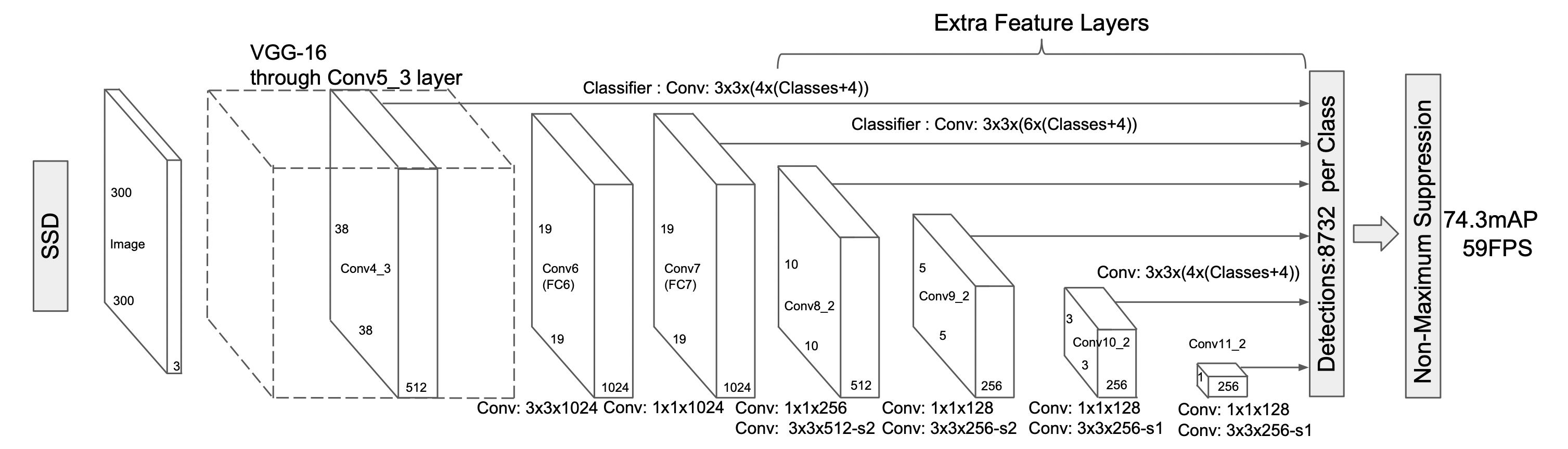
SSD는 base network와 auxiliary structure network로 이루어진 1-stage detector 입니다.
VGG-16 network를 base network로 사용하였고, auxiliary structure network로 Convolutional network를 사용하였습니다.
SSD는 VGG-16 network에서 많은 파라미터를 요구하는 fc레이어를 사용하지 않고 convolution layer로 대체하여 base network와 auxiliary structure network를 연결하였습니다.

Multi-scale feature maps for detection

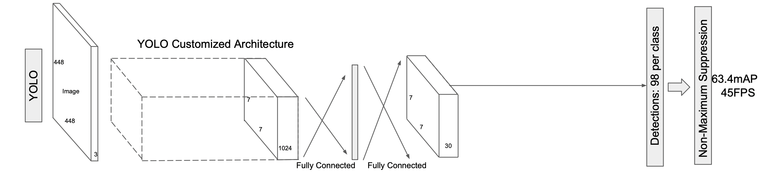
YOLO의 7×7 single scale feature map과는 다르게 multi-scale feature maps을 사용하였습니다.
Base network의 마지막 부분에 convolution layer들을 추가하는데, 해당 layer들은 점진적으로 size가 감소하며, 이는 다양한 scale에 대해 뛰어난 detection 성능을 만들어냅니다.

• 논문에서는 6종류의 scale을 가지는 feature maps를 사용하였습니다. (38×38, 19×19, 10×10, 5×5, 3×3, 1×1)

Convolutional predictors for detection

pchannels를 갖는 m×n의 feature map에 3×3×p크기의 convolution filter를 적용하였습니다.
Detection(Output)은 default bounding boxes의 category score와 box offsets을 측정합니다.
SSD는 Detection까지 convolution 연산을 하는 반면, YOLO는 fc 연산을 거치기 때문에 연산량과 속도 측면에서 효과적이였습니다.

Default boxes and aspect ratios

각각의 feature map cell마다 서로 다른 크기의 scale과 aspect ratio(종횡비)를 가지는 default box를 생성합니다. [Default boxes는 Faster R-CNN의 anchor boxes와 비슷합니다. 하지만 6종류의 scale을 가진 feature map의 각각의 cell마다 default boxes를 생성한다는 점이 다릅니다.]
각각의 cell은 (c+4)k 개의 예측을 합니다. c는 class 수를, k는 default boxes의 개수를, 4는 4개의 offset를 의미합니다. 이를 m×nfeature map에 적용하면 (c+4)k m n 개의 output이 출력됩니다.

2. Training

Matching strategy

Training을 진행하기위해 default boxes를 ground truth와 매칭합니다. 본 논문에서는 jaccard overlap(또는 Intersection Over UnionIOU)값이 0.5 이상인 boxes들을 positive(Object가 있는/negative는 Object가 없는. 즉 배경을 의미) boxes로 사용합니다.

Training objective

Loss function은 localization loss(loc) 와 confidence loss(conf)의 가중 합 입니다.

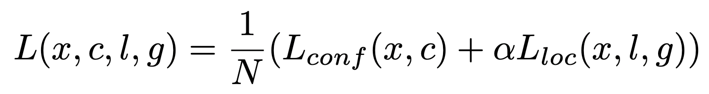
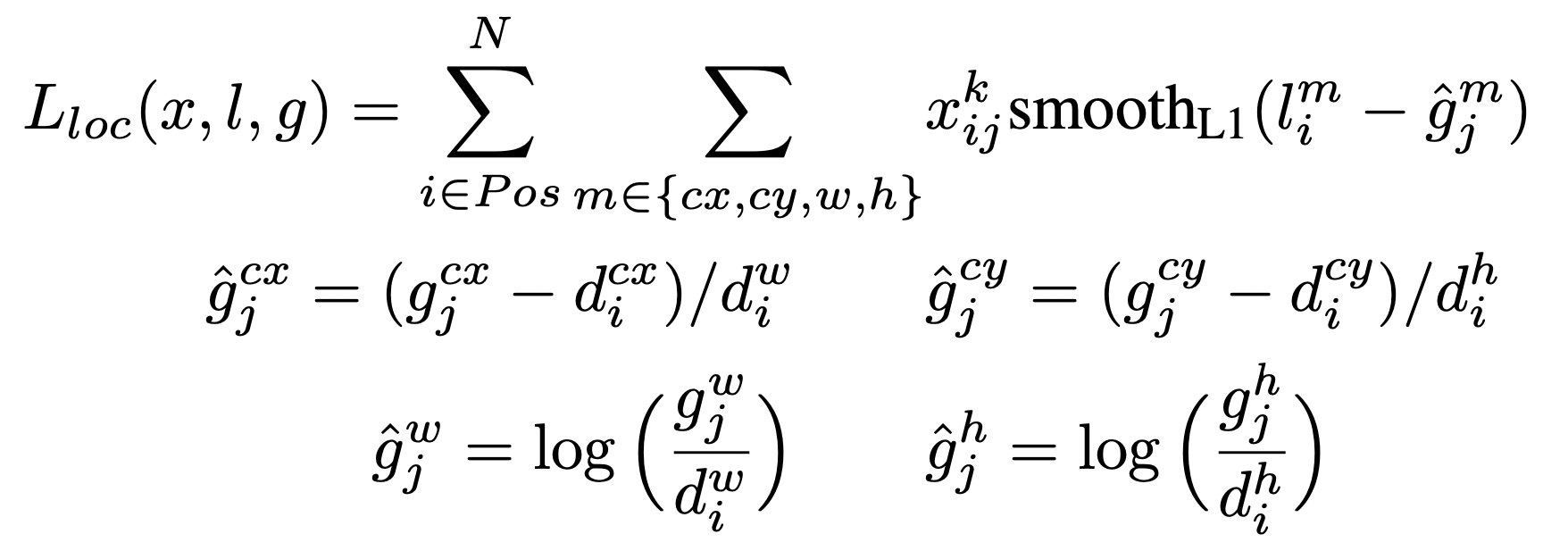
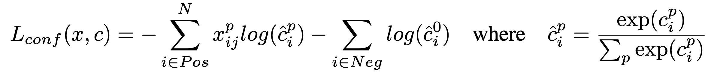
• N: number of matched default boxes
• x_ij^p = {1, 0}: indicator for matching the i-th default box to the j-th ground truth box of category p / positive box = 1, negative box = 0
• l: predicted box
• g: ground truth box
• d: default box
• cx, cy: center x, y
• w: width
• h: height
• a: 1

Choosing scales and aspect ratios for default boxes

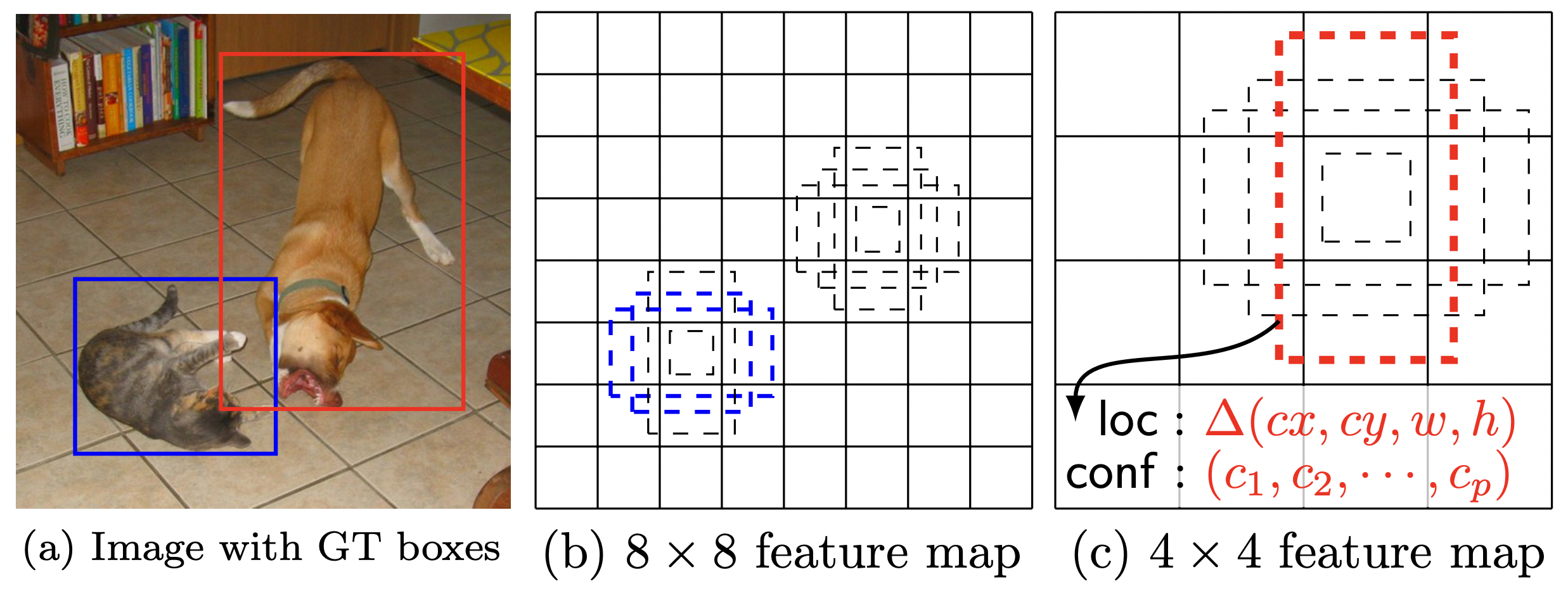
위 그림의 (b)와 (c)를 보면 feature map의 크기가 작아질수록 더 큰 object detection이 가능함을 알 수 있습니다.

본 논문에서는 이러한 default box의 scale을 다음과 같이 정의합니다.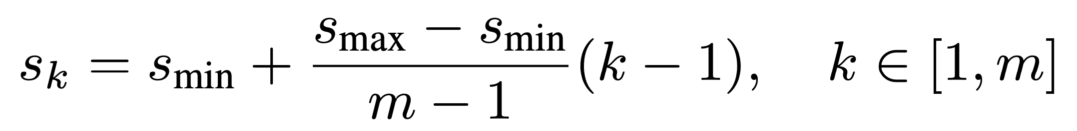

• m: Number of scale feature map (6)
  s<sub>k</sub>값은 원본 이미지에 대한 비율을 의미하며, 해당 수식을 통해 다양한 크기의 default box를 생성할 수 있습니다.

ex) 300×300 원본 이미지에 대하여 s = 0.1이고 aspect ratio가 1:1이면 default box의 size는 30×30이 됩니다.

Hard negative mining

이미지를 생각해보면 object보다 background의 비중이 훨씬 높을겁니다. 이러한 상황을 반영하여 positive와 negative의 비율을 1:3으로 하여 데이터를 사용합니다.

Data augmentation

Robust한 모델을 얻기 위하여 data augmentation을 수행하였습니다.

Result from the Paper

PASCAL VOC, COCO datasets에서 속도(FPS)와 정확도(mAP)가 가장 높은 모델이였습니다. (16년도 기준)
아래표에서 Fast YOLO는 2017에 제안된 논문으로 정확도를 포기하고 속도에만 중점을 둔 모델입니다.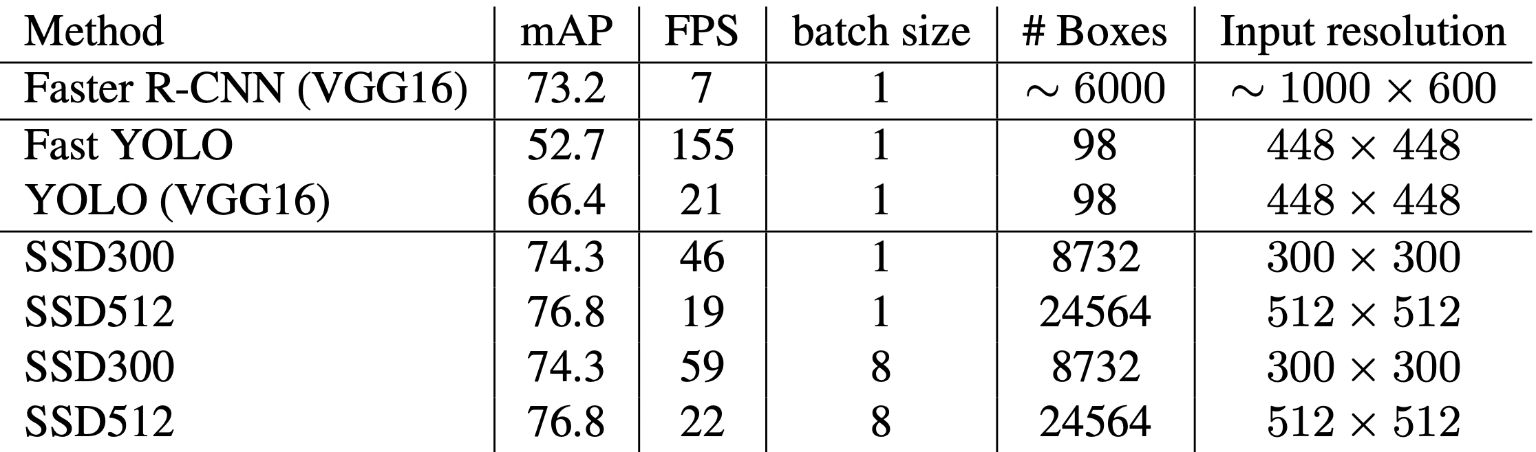

최근에 제안된 YOLO(single-scale)나 Swin(mulit-scale)에게 처참히 밀려있는 근황입니다.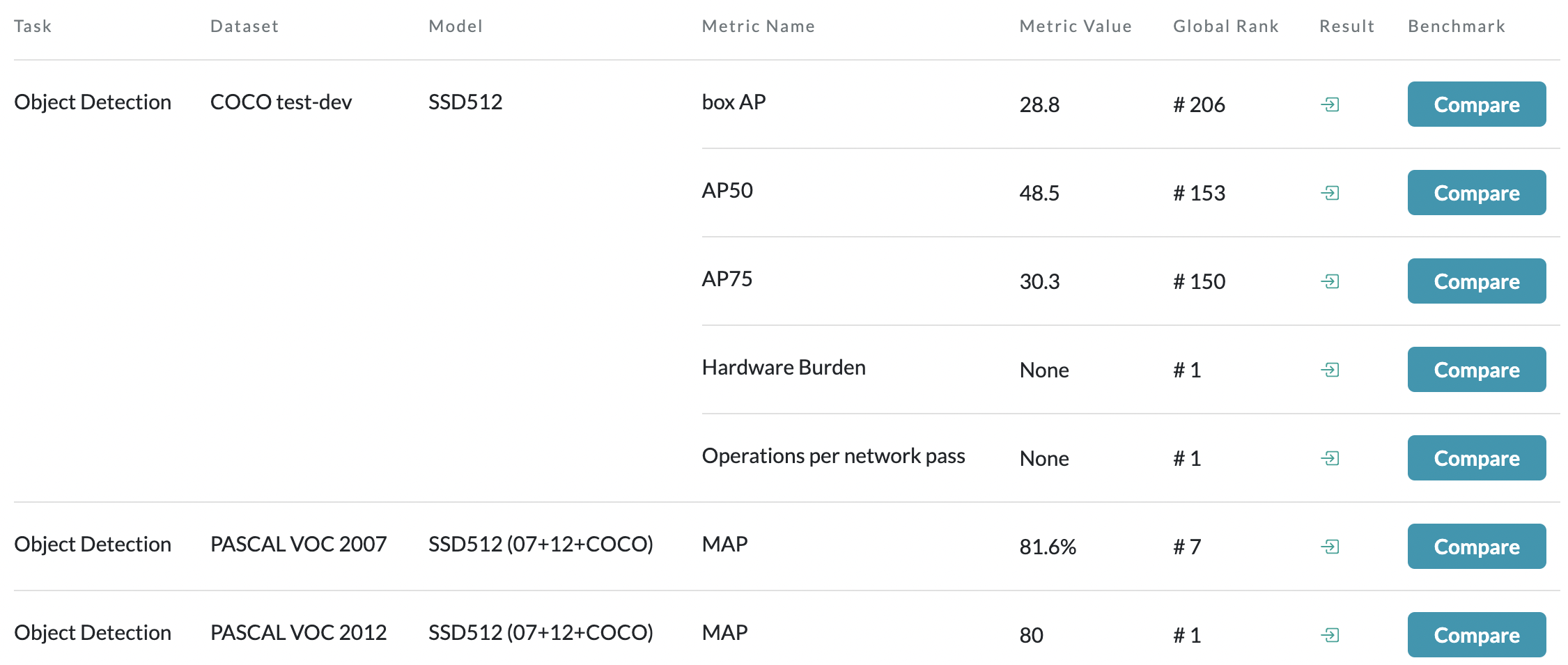

SSD 모델 사용해보기

Pytorch Hub - SSD를 이용하여 쉽고 빠르게 모델을 불러와서 사용해볼 수 있었습니다.

import torch
ssd_model = torch.hub.load('NVIDIA/DeepLearningExamples:torchhub', 'nvidia_ssd')
utils = torch.hub.load('NVIDIA/DeepLearningExamples:torchhub', 'nvidia_ssd_processing_utils')

Downloading: "https://download.pytorch.org/models/resnet50-0676ba61.pth" to /root/.cache/torch/hub/checkpoints/resnet50-0676ba61.pth

97.8M/97.8M [00:00<00:00, 143MB/s] Downloading checkpoint from https://api.ngc.nvidia.com/v2/models/nvidia/ssd_pyt_ckpt_amp/versions/20.06.0/files/nvidia_ssdpyt_amp_200703.pt Using cache found in /root/.cache/torch/hub/NVIDIA_DeepLearningExamples_torchhub

사전에 훈련된 SSD 모델과 유틸리티 파일들을 torch-hub를 통해 쉽게 불러올 수 있습니다.

ssd_model.to('cuda')
ssd_model.eval()

SSD300(

(feature_extractor): ResNet( (feature_extractor): Sequential( (0): Conv2d(3, 64, kernel_size=(7, 7), stride=(2, 2), padding=(3, 3), bias=False) (1): BatchNorm2d(64, eps=1e-05, momentum=0.1, affine=True, track_running_stats=True) (2): ReLU(inplace=True) (3): MaxPool2d(kernel_size=3, stride=2, padding=1, dilation=1, ceil_mode=False) (4): Sequential( (0): Bottleneck( (conv1): Conv2d(64, 64, kernel_size=(1, 1), stride=(1, 1), bias=False) (bn1): BatchNorm2d(64, eps=1e-05, momentum=0.1, affine=True, track_running_stats=True) (conv2): Conv2d(64, 64, kernel_size=(3, 3), stride=(1, 1), padding=(1, 1), bias=False) (bn2): BatchNorm2d(64, eps=1e-05, momentum=0.1, affine=True, track_running_stats=True) (conv3): Conv2d(64, 256, kernel_size=(1, 1), stride=(1, 1), bias=False) (bn3): BatchNorm2d(256, eps=1e-05, momentum=0.1, affine=True, track_running_stats=True) (relu): ReLU(inplace=True) (downsample): Sequential( (0): Conv2d(64, 256, kernel_size=(1, 1), stride=(1, 1), bias=False) (1): BatchNorm2d(256, eps=1e-05, momentum=0.1, affine=True, track_running_stats=True) ) ) (1): Bottleneck( (conv1): Conv2d(256, 64, kernel_size=(1, 1), stride=(1, 1), bias=False) (bn1): BatchNorm2d(64, eps=1e-05, momentum=0.1, affine=True, track_running_stats=True) (conv2): Conv2d(64, 64, kernel_size=(3, 3), stride=(1, 1), padding=(1, 1), bias=False) (bn2): BatchNorm2d(64, eps=1e-05, momentum=0.1, affine=True, track_running_stats=True) (conv3): Conv2d(64, 256, kernel_size=(1, 1), stride=(1, 1), bias=False) (bn3): BatchNorm2d(256, eps=1e-05, momentum=0.1, affine=True, track_running_stats=True) (relu): ReLU(inplace=True) ) (2): Bottleneck( (conv1): Conv2d(256, 64, kernel_size=(1, 1), stride=(1, 1), bias=False) (bn1): BatchNorm2d(64, eps=1e-05, momentum=0.1, affine=True, track_running_stats=True) (conv2): Conv2d(64, 64, kernel_size=(3, 3), stride=(1, 1), padding=(1, 1), bias=False) (bn2): BatchNorm2d(64, eps=1e-05, momentum=0.1, affine=True, track_running_stats=True) (conv3): Conv2d(64, 256, kernel_size=(1, 1), stride=(1, 1), bias=False) (bn3): BatchNorm2d(256, eps=1e-05, momentum=0.1, affine=True, track_running_stats=True) (relu): ReLU(inplace=True) ) ) (5): Sequential( (0): Bottleneck( (conv1): Conv2d(256, 128, kernel_size=(1, 1), stride=(1, 1), bias=False) (bn1): BatchNorm2d(128, eps=1e-05, momentum=0.1, affine=True, track_running_stats=True) (conv2): Conv2d(128, 128, kernel_size=(3, 3), stride=(2, 2), padding=(1, 1), bias=False) (bn2): BatchNorm2d(128, eps=1e-05, momentum=0.1, affine=True, track_running_stats=True) (conv3): Conv2d(128, 512, kernel_size=(1, 1), stride=(1, 1), bias=False) (bn3): BatchNorm2d(512, eps=1e-05, momentum=0.1, affine=True, track_running_stats=True) (relu): ReLU(inplace=True) (downsample): Sequential( (0): Conv2d(256, 512, kernel_size=(1, 1), stride=(2, 2), bias=False) (1): BatchNorm2d(512, eps=1e-05, momentum=0.1, affine=True, track_running_stats=True) ) ) (1): Bottleneck( (conv1): Conv2d(512, 128, kernel_size=(1, 1), stride=(1, 1), bias=False) (bn1): BatchNorm2d(128, eps=1e-05, momentum=0.1, affine=True, track_running_stats=True) (conv2): Conv2d(128, 128, kernel_size=(3, 3), stride=(1, 1), padding=(1, 1), bias=False) (bn2): BatchNorm2d(128, eps=1e-05, momentum=0.1, affine=True, track_running_stats=True) (conv3): Conv2d(128, 512, kernel_size=(1, 1), stride=(1, 1), bias=False) (bn3): BatchNorm2d(512, eps=1e-05, momentum=0.1, affine=True, track_running_stats=True) (relu): ReLU(inplace=True) ) (2): Bottleneck( (conv1): Conv2d(512, 128, kernel_size=(1, 1), stride=(1, 1), bias=False) (bn1): BatchNorm2d(128, eps=1e-05, momentum=0.1, affine=True, track_running_stats=True) (conv2): Conv2d(128, 128, kernel_size=(3, 3), stride=(1, 1), padding=(1, 1), bias=False) (bn2): BatchNorm2d(128, eps=1e-05, momentum=0.1, affine=True, track_running_stats=True) (conv3): Conv2d(128, 512, kernel_size=(1, 1), stride=(1, 1), bias=False) (bn3): BatchNorm2d(512, eps=1e-05, momentum=0.1, affine=True, track_running_stats=True) (relu): ReLU(inplace=True) ) (3): Bottleneck( (conv1): Conv2d(512, 128, kernel_size=(1, 1), stride=(1, 1), bias=False) (bn1): BatchNorm2d(128, eps=1e-05, momentum=0.1, affine=True, track_running_stats=True) (conv2): Conv2d(128, 128, kernel_size=(3, 3), stride=(1, 1), padding=(1, 1), bias=False) (bn2): BatchNorm2d(128, eps=1e-05, momentum=0.1, affine=True, track_running_stats=True) (conv3): Conv2d(128, 512, kernel_size=(1, 1), stride=(1, 1), bias=False) (bn3): BatchNorm2d(512, eps=1e-05, momentum=0.1, affine=True, track_running_stats=True) (relu): ReLU(inplace=True) ) ) (6): Sequential( (0): Bottleneck( (conv1): Conv2d(512, 256, kernel_size=(1, 1), stride=(1, 1), bias=False) (bn1): BatchNorm2d(256, eps=1e-05, momentum=0.1, affine=True, track_running_stats=True) (conv2): Conv2d(256, 256, kernel_size=(3, 3), stride=(1, 1), padding=(1, 1), bias=False) (bn2): BatchNorm2d(256, eps=1e-05, momentum=0.1, affine=True, track_running_stats=True) (conv3): Conv2d(256, 1024, kernel_size=(1, 1), stride=(1, 1), bias=False) (bn3): BatchNorm2d(1024, eps=1e-05, momentum=0.1, affine=True, track_running_stats=True) (relu): ReLU(inplace=True) (downsample): Sequential( (0): Conv2d(512, 1024, kernel_size=(1, 1), stride=(1, 1), bias=False) (1): BatchNorm2d(1024, eps=1e-05, momentum=0.1, affine=True, track_running_stats=True) ) ) (1): Bottleneck( (conv1): Conv2d(1024, 256, kernel_size=(1, 1), stride=(1, 1), bias=False) (bn1): BatchNorm2d(256, eps=1e-05, momentum=0.1, affine=True, track_running_stats=True) (conv2): Conv2d(256, 256, kernel_size=(3, 3), stride=(1, 1), padding=(1, 1), bias=False) (bn2): BatchNorm2d(256, eps=1e-05, momentum=0.1, affine=True, track_running_stats=True) (conv3): Conv2d(256, 1024, kernel_size=(1, 1), stride=(1, 1), bias=False) (bn3): BatchNorm2d(1024, eps=1e-05, momentum=0.1, affine=True, track_running_stats=True) (relu): ReLU(inplace=True) ) (2): Bottleneck( (conv1): Conv2d(1024, 256, kernel_size=(1, 1), stride=(1, 1), bias=False) (bn1): BatchNorm2d(256, eps=1e-05, momentum=0.1, affine=True, track_running_stats=True) (conv2): Conv2d(256, 256, kernel_size=(3, 3), stride=(1, 1), padding=(1, 1), bias=False) (bn2): BatchNorm2d(256, eps=1e-05, momentum=0.1, affine=True, track_running_stats=True) (conv3): Conv2d(256, 1024, kernel_size=(1, 1), stride=(1, 1), bias=False) (bn3): BatchNorm2d(1024, eps=1e-05, momentum=0.1, affine=True, track_running_stats=True) (relu): ReLU(inplace=True) ) (3): Bottleneck( (conv1): Conv2d(1024, 256, kernel_size=(1, 1), stride=(1, 1), bias=False) (bn1): BatchNorm2d(256, eps=1e-05, momentum=0.1, affine=True, track_running_stats=True) (conv2): Conv2d(256, 256, kernel_size=(3, 3), stride=(1, 1), padding=(1, 1), bias=False) (bn2): BatchNorm2d(256, eps=1e-05, momentum=0.1, affine=True, track_running_stats=True) (conv3): Conv2d(256, 1024, kernel_size=(1, 1), stride=(1, 1), bias=False) (bn3): BatchNorm2d(1024, eps=1e-05, momentum=0.1, affine=True, track_running_stats=True) (relu): ReLU(inplace=True) ) (4): Bottleneck( (conv1): Conv2d(1024, 256, kernel_size=(1, 1), stride=(1, 1), bias=False) (bn1): BatchNorm2d(256, eps=1e-05, momentum=0.1, affine=True, track_running_stats=True) (conv2): Conv2d(256, 256, kernel_size=(3, 3), stride=(1, 1), padding=(1, 1), bias=False) (bn2): BatchNorm2d(256, eps=1e-05, momentum=0.1, affine=True, track_running_stats=True) (conv3): Conv2d(256, 1024, kernel_size=(1, 1), stride=(1, 1), bias=False) (bn3): BatchNorm2d(1024, eps=1e-05, momentum=0.1, affine=True, track_running_stats=True) (relu): ReLU(inplace=True) ) (5): Bottleneck( (conv1): Conv2d(1024, 256, kernel_size=(1, 1), stride=(1, 1), bias=False) (bn1): BatchNorm2d(256, eps=1e-05, momentum=0.1, affine=True, track_running_stats=True) (conv2): Conv2d(256, 256, kernel_size=(3, 3), stride=(1, 1), padding=(1, 1), bias=False) (bn2): BatchNorm2d(256, eps=1e-05, momentum=0.1, affine=True, track_running_stats=True) (conv3): Conv2d(256, 1024, kernel_size=(1, 1), stride=(1, 1), bias=False) (bn3): BatchNorm2d(1024, eps=1e-05, momentum=0.1, affine=True, track_running_stats=True) (relu): ReLU(inplace=True) ) ) ) ) (additional_blocks): ModuleList( (0): Sequential( (0): Conv2d(1024, 256, kernel_size=(1, 1), stride=(1, 1), bias=False) (1): BatchNorm2d(256, eps=1e-05, momentum=0.1, affine=True, track_running_stats=True) (2): ReLU(inplace=True) (3): Conv2d(256, 512, kernel_size=(3, 3), stride=(2, 2), padding=(1, 1), bias=False) (4): BatchNorm2d(512, eps=1e-05, momentum=0.1, affine=True, track_running_stats=True) (5): ReLU(inplace=True) ) (1): Sequential( (0): Conv2d(512, 256, kernel_size=(1, 1), stride=(1, 1), bias=False) (1): BatchNorm2d(256, eps=1e-05, momentum=0.1, affine=True, track_running_stats=True) (2): ReLU(inplace=True) (3): Conv2d(256, 512, kernel_size=(3, 3), stride=(2, 2), padding=(1, 1), bias=False) (4): BatchNorm2d(512, eps=1e-05, momentum=0.1, affine=True, track_running_stats=True) (5): ReLU(inplace=True) ) (2): Sequential( (0): Conv2d(512, 128, kernel_size=(1, 1), stride=(1, 1), bias=False) (1): BatchNorm2d(128, eps=1e-05, momentum=0.1, affine=True, track_running_stats=True) (2): ReLU(inplace=True) (3): Conv2d(128, 256, kernel_size=(3, 3), stride=(2, 2), padding=(1, 1), bias=False) (4): BatchNorm2d(256, eps=1e-05, momentum=0.1, affine=True, track_running_stats=True) (5): ReLU(inplace=True) ) (3): Sequential( (0): Conv2d(256, 128, kernel_size=(1, 1), stride=(1, 1), bias=False) (1): BatchNorm2d(128, eps=1e-05, momentum=0.1, affine=True, track_running_stats=True) (2): ReLU(inplace=True) (3): Conv2d(128, 256, kernel_size=(3, 3), stride=(1, 1), bias=False) (4): BatchNorm2d(256, eps=1e-05, momentum=0.1, affine=True, track_running_stats=True) (5): ReLU(inplace=True) ) (4): Sequential( (0): Conv2d(256, 128, kernel_size=(1, 1), stride=(1, 1), bias=False) (1): BatchNorm2d(128, eps=1e-05, momentum=0.1, affine=True, track_running_stats=True) (2): ReLU(inplace=True) (3): Conv2d(128, 256, kernel_size=(3, 3), stride=(1, 1), bias=False) (4): BatchNorm2d(256, eps=1e-05, momentum=0.1, affine=True, track_running_stats=True) (5): ReLU(inplace=True) ) ) (loc): ModuleList( (0): Conv2d(1024, 16, kernel_size=(3, 3), stride=(1, 1), padding=(1, 1)) (1): Conv2d(512, 24, kernel_size=(3, 3), stride=(1, 1), padding=(1, 1)) (2): Conv2d(512, 24, kernel_size=(3, 3), stride=(1, 1), padding=(1, 1)) (3): Conv2d(256, 24, kernel_size=(3, 3), stride=(1, 1), padding=(1, 1)) (4): Conv2d(256, 16, kernel_size=(3, 3), stride=(1, 1), padding=(1, 1)) (5): Conv2d(256, 16, kernel_size=(3, 3), stride=(1, 1), padding=(1, 1)) ) (conf): ModuleList( (0): Conv2d(1024, 324, kernel_size=(3, 3), stride=(1, 1), padding=(1, 1)) (1): Conv2d(512, 486, kernel_size=(3, 3), stride=(1, 1), padding=(1, 1)) (2): Conv2d(512, 486, kernel_size=(3, 3), stride=(1, 1), padding=(1, 1)) (3): Conv2d(256, 486, kernel_size=(3, 3), stride=(1, 1), padding=(1, 1)) (4): Conv2d(256, 324, kernel_size=(3, 3), stride=(1, 1), padding=(1, 1)) (5): Conv2d(256, 324, kernel_size=(3, 3), stride=(1, 1), padding=(1, 1)) ) )

GPU를 사용할 수 있도록 지정해주고, 불러온 모델을 확인해봅니다.

앞에서 읽은 논문과는 다르게 base network가 VGG-16이 아닌 ResNet-50인것을 확인할 수 있습니다.

논문에서 We use the VGG-16 network as a base, but other networks should also produce good results.라는 내용이 있었는데, base network를 성능이 더 좋은 ResNet을 사용한 것이라고 생각하고 넘어갔습니다.
(사실 코랩의 Model Description이나 파이토치 허브에서 ResNet를 사용한다고 설명하지만, 앞에서 논문 읽고 분석한걸 생색내려고 쓴 말입니다 ><)

uris = [
    'http://images.cocodataset.org/val2017/000000397133.jpg',
    'http://images.cocodataset.org/val2017/000000037777.jpg',
    'http://images.cocodataset.org/val2017/000000252219.jpg'
]

Object Detection을 위한 테스트 이미지를 준비합니다.

inputs = [utils.prepare_input(uri) for uri in uris]
tensor = utils.prepare_tensor(inputs)

network의 input에 맞게 이미지를 포멧하고 텐서로 변환합니다.

SSD300 모델이므로 input shape는 (300, 300, 3).

with torch.no_grad():
    detections_batch = ssd_model(tensor)

SSD모델을 통해 object detection을 수행합니다.

results_per_input = utils.decode_results(detections_batch)
best_results_per_input = [utils.pick_best(results, 0.40) for results in results_per_input]

신뢰도가 40% 이상인 reasonable한 detections의 정보만 가져옵니다.

classes_to_labels = utils.get_coco_object_dictionary()

Class ID를 object name으로 매핑하기 위한 dictionary를 다운받습니다.

from matplotlib import pyplot as plt
import matplotlib.patches as patches

for image_idx in range(len(best_results_per_input)):
    fig, ax = plt.subplots(1)
    # Show original, denormalized image...
    image = inputs[image_idx] / 2 + 0.5
    ax.imshow(image)
    # ...with detections
    bboxes, classes, confidences = best_results_per_input[image_idx]
    for idx in range(len(bboxes)):
        left, bot, right, top = bboxes[idx]
        x, y, w, h = [val * 300 for val in [left, bot, right - left, top - bot]]
        rect = patches.Rectangle((x, y), w, h, linewidth=1, edgecolor='r', facecolor='none')
        ax.add_patch(rect)
        ax.text(x, y, "{} {:.0f}%".format(classes_to_labels[classes[idx] - 1], confidences[idx]*100), bbox=dict(facecolor='white', alpha=0.5))
plt.show()

결과 이미지 확인하기

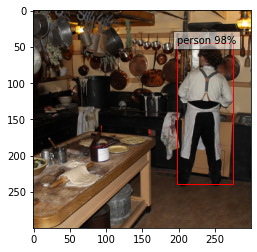
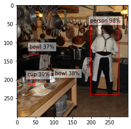
결과 이미지 확인하기를 누르면 두개의 이미지가 보일 것입니다.

첫번째는 신뢰도가 40% 이상인 object를 시각화한 사진이며, 두번째는 신뢰도가 30% 이상인 object를 시각화한 사진입니다.

또한 실제로는 다른 상황의 이미지 3종류에 대한 detection 결과를 확인할 수 있으나, 신뢰도 값을 변경하였을때 가장 큰 변화가 일어난 이미지 1종류에 대한 비교만 결과에 넣어놓았습니다.

마무리

이렇게 SSD 논문에 대하여 읽고 분석해보았으며, 파이토치 허브를 통하여 쉽고 간단하게 학습된 모델을 불러와 사용해볼 수 있었습니다. 모델 training 시간을 생략할 수 있으며, 논문을 읽고나서 바로 Remind 해볼 수 있어서 좋았습니다. 파이토치 허브 커뮤니티가 커져서 더 다양한 모델들이 추가된다면 공부하는 사람들에게 많은 도움이 될 것 같습니다.